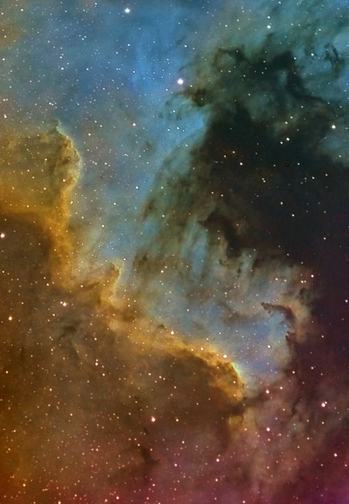


Recently I began to take astronomical pictures in narrow band using my SBIG ST2000XM and a set of Baader Filters (Hα, Hb, OIII and SII).
One of the most famous color composition technique of narrowband data is the Hubble Palette that gives to nebulas a typical golden-turquoise color palette.
In this composition the SII emission is associated to Red, OII to Blue and H alpha to Green.
The drawback of this composition is that, since Hα widely dominates on OIII and SII emission, OIII and SII image histograms should be boosted relative to Hα, this bloats stars and creates weird magenta halos.
To overcome this problem J-P Metsavainio has developed a technique based on tone maps, starless copies of the original narrowband channels, and an enhanced luminance based on Hα image modified with OIII and SII tone maps.
Using starless copies allows boosting faint channels without worrying about stars; moreover the noisy OIII and SII channels can be strongly denoised as they will be used only for chrominance: all the details will be in the enhanced Hα luminance.
The original Metsavainio method is based on Photoshop; I will try to translate the workflow in PixInsight with only a few differences.
The data set
The data set used for this tutorial consists in images of the Mexico Gulf in NGC 7000 taken with a SBIG ST2000XM camera equipped with a Baader filter set:
Hα 7 nm
OIII 8.5 nm
SII 8 nm
on a TS 80 Q refractor under a suburban sky.
Hereafter Ha will be the master Hα image: Oiii the master OIII image and Sii the master SII, all at linear stage.
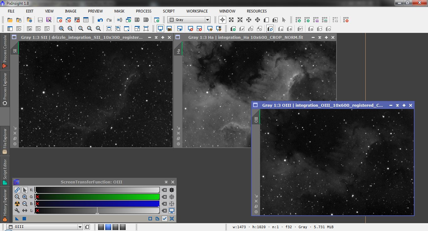
Creating the tone maps
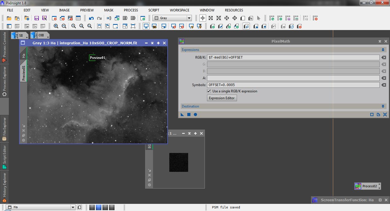
The starting images should be perfectly registered, gradient free and, possibly, with the same background level. To do this use DynamicBackgroundExtractor if gradients are present, then use PixelMath to set all the backgrounds to the same level: create a small preview containing only background, drag its tab on the PixInsight Working area to create a new image and rename it to BG.
Open PixelMath and write the following expression.
$T-med(BG)+OFFSETthe function med() calculates the median value of the image (representative of the background level); OFFSET is the desired new background (I usually set it at 0.0005): remember this value, we will need it later in the workflow.
You can simply replace OFFSET with the desired value in the expression or define a symbol.
Repeat on all the images using the same area of sky (use Propagate previews script to replicate the preview on the other images).
In the original technique Metsavainio uses an already stretched (nonlinear) copy of the images to create the tone maps, probably because Photoshop doesn't have a Screen Transfer Function feature so it's almost impossible to work on linear images because they are barely visible; PixInsight has such a feature so I prefer to remain at linear stage as long as possible.
The basic technique to produce a starless copy of an image consists in creating a star mask, protecting the background and the nebular details, and use a combination of MultiscaleMedianTransform, to remove High frequency details, and MorphologicalTransformation to reduce the residuals.
Since StarMask seems to work better on nonlinear images, create a copy of the image and apply an HistogramTransformation to show clearly all the stars.
If strong nonstellar signal is present use an aggressive HDRMultiscaleTransform (low scale, 2 or 3 iterations), than try to create a star mask that covers all the stars present, for this task it's better to check "binarize" option on the StarMask process.
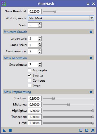
Sometimes StarMask process misrecognize high contrast nebular structures as stars, if it happens correct the star mask with the CloneStamp deleting the fake stars.
When the mask is ready make a copy of the first image, rename it adding the _TM suffix to identify it as a Tone Map and apply the star mask; open MultiscaleMedianTransform , remove the first 5 or 6 wavelet layers and apply it dragging the blue triangle icon on the image; If hint of stars are still present you can try again with MMT or with MorphologicalTransformation using then erosion process.
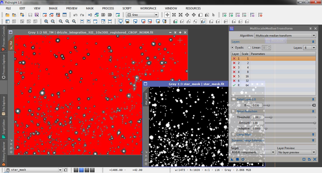
When done repeat the workflow on the remaining images using the same star mask: now you should have three linear tone maps (let's say Ha_TM, Oiii_TM, Sii_TM).
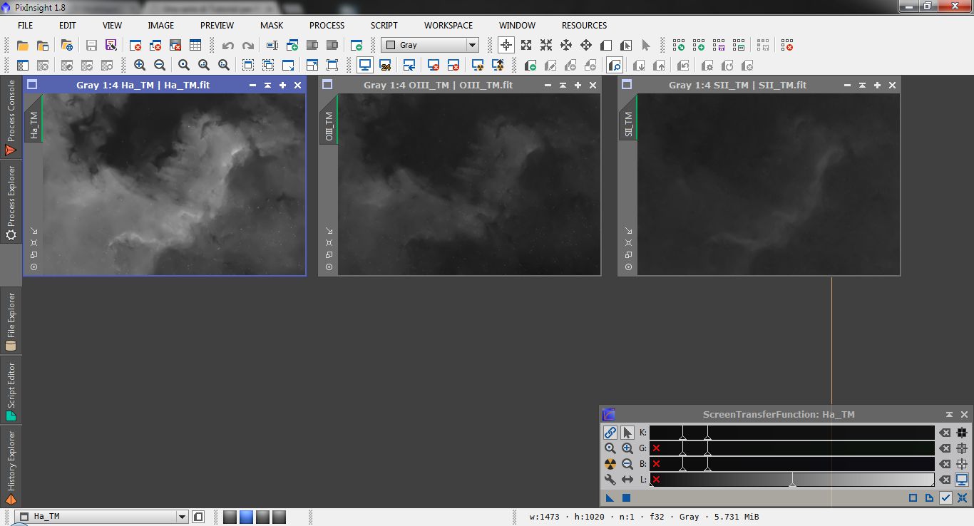
This tone maps, the fainter channels in particular, may contain a lot of noise; PixInsight has different denoise tools that works well on linear images.
The perfect tool for this job is TGVDenoise: combined with a Local support it can apply a very strong denoise without losing details in the high S/N parts.
Create a small preview on the background sky and, using Statistic process, evaluate the standard deviation of the background signal: since I want an aggressive denoise the first guess value for the edge protection parameter will be twice (or more) the standard deviation.
Apply the Local support with the standard settings except the shadow set slightly higher than the OFFSET value, set the iterations parameter to 400 or higher than apply the process to a small preview containing both sky background and nebula details.
Trim the strength parameter to get the desired amount of denoise: if important structures in the nebula disappear lower the edge protection parameter, if noise "structures" survive on the background increase it.
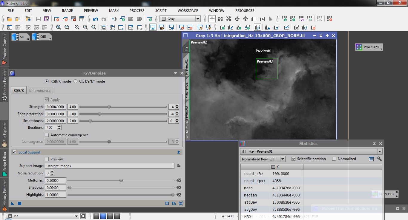
When the best parameters are found apply the process to the whole image.
Repeat the procedure on the three narrow band channels.
Creating the enhanced Luminance
As explained by Metsavainio in his tutorial the Hα channel does not fully represent luminance because it lacks information about OIII and SII distribution: he enhance the Hα channel using OIII and SII tone maps.
The simplest way to do is simply add the tone maps to the Hα with PixelMath using the expression
$T+Oiii_TM-OFFSET+Sii_TM-OFFSET (or briefly $T+Oiii_TM+Sii_TM-2*OFFSET)OFFSET is the same value used before: drag and drop the blue triangle on the original Hα image to create the Enhanced Luminance (still linear).
A better, and more rigorous, way to compose the images is to take into account the differences between exposures, binning and Quantum efficiency of the CCD.
Given that the images are correctly calibrated, the composition can be done easily with PixelMath defining a few Symbols:
- HaBIN: H alpha binning
- HaEXP: H alpha exposure
- HaQE H alpha quantum efficiency of the CCD (in the range 0-1)
- OiiiBIN: OIII binning
- OiiiEXP: OIII exposure
- OiiiQE OIII quantum efficiency of the CCD (in the range 0-1)
- SiiBIN: SII binning
- SiiEXP: SII exposure
- SiiQE SII quantum efficiency of the CCD (in the range 0-1)
- OFFSET The offset used before for background equalization
Assuming that the operation will be applied to the Hα image the expression is
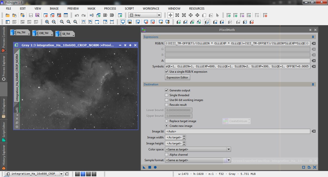
In both cases ,if some Highlight clipping occurs, activate the "rescale" flag. This expression corrects for differences between channels and create a luminance with the correct ratios.
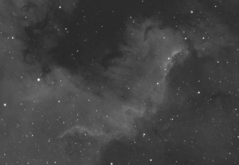
Mouseover to see before-after Luminance enhancement
Creating the RGB tone map
It's now time to join the single tone maps to get the RGB tone map: as said before the Hα signal is usually dominant so, simply creating and RGB image from the tone maps would lead, in Hubble palette, a completely green image.
In the original method Metsavainio enhance the visibility of OIII and SII signal through a sequence of Histogram and curves transformations with the goal to equalize the luminosity of OIII and SII images with the Hα, then merge the channels in an RGB image and trim the colors giving to the image his legendary touch.
Since tone maps in my method are linear I prefer to apply only linear transformations: to equalize the luminosity I use LinearFit process using the Hα tone map as reference and applying it to SII and OIII tone maps; when done I simply create and RGB (linear) image with ChannelCombination process using Sii_TM as red, Ha_TM as green and Oiii_TM as blue.
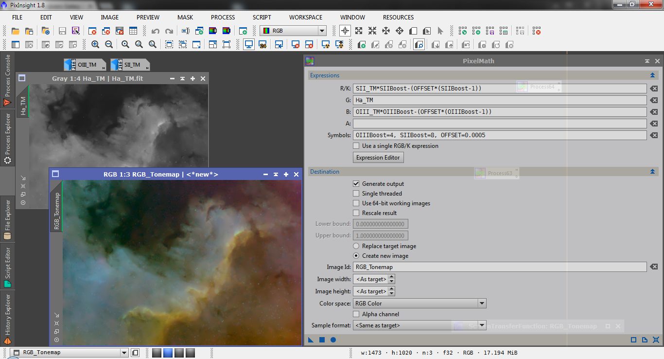
If one prefers to have better control on color composition can use PixelMath for the composition using "boosting factors" for OIII and SII:
| Red | Sii_TM*SIIBoost-(SIIBoost-1)*OFFSET |
| Green | Ha_TM |
| Blue | Oiii_TM*OIIIBoost-( OIIIBoost -1)*OFFSET |
| Symbols | SIIBoost=7; OIIIBoost=4; OFFSET=0.0005 |
Trimming SIIBoost and OIIIBoost the desired color balance can be achieved.
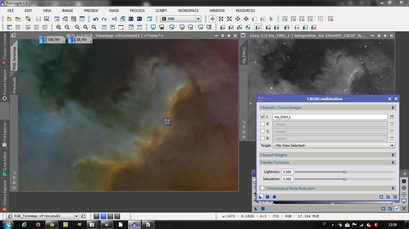
Composing the final image
The final composition of the image is a usual LRGB composition using the enhanced luminance as L channel and the color Tone Map as RGB.
Since the images are still linear should be stretched before LRGB composing.
I usually use Deconvolution, and TGVDenoise on the linear Luminance than I make a nonlinear stretching with HistogramTansformation or MaskedStretch and fine tune with CurvesTransformation.
Then I do a similar nonlinear stretching on the RGB.
When achieved the desired look open the LRGBComposition process, select the enhanced luminance as L channel, disable R,G,B checkboxes and Drag and drop the blue triangle over the color tone map: The lightness will be applied to the RGB, fine tune the image with whichever process you are used to and enjoy your hard work.
Mouse over for the before-after application of luminance

Here the final result of the processing, click on the image for the full res version on AstroBin