Leggilo in italiano

I recently participated in an astrophotography processing contest promoted by Martin Liersch website.

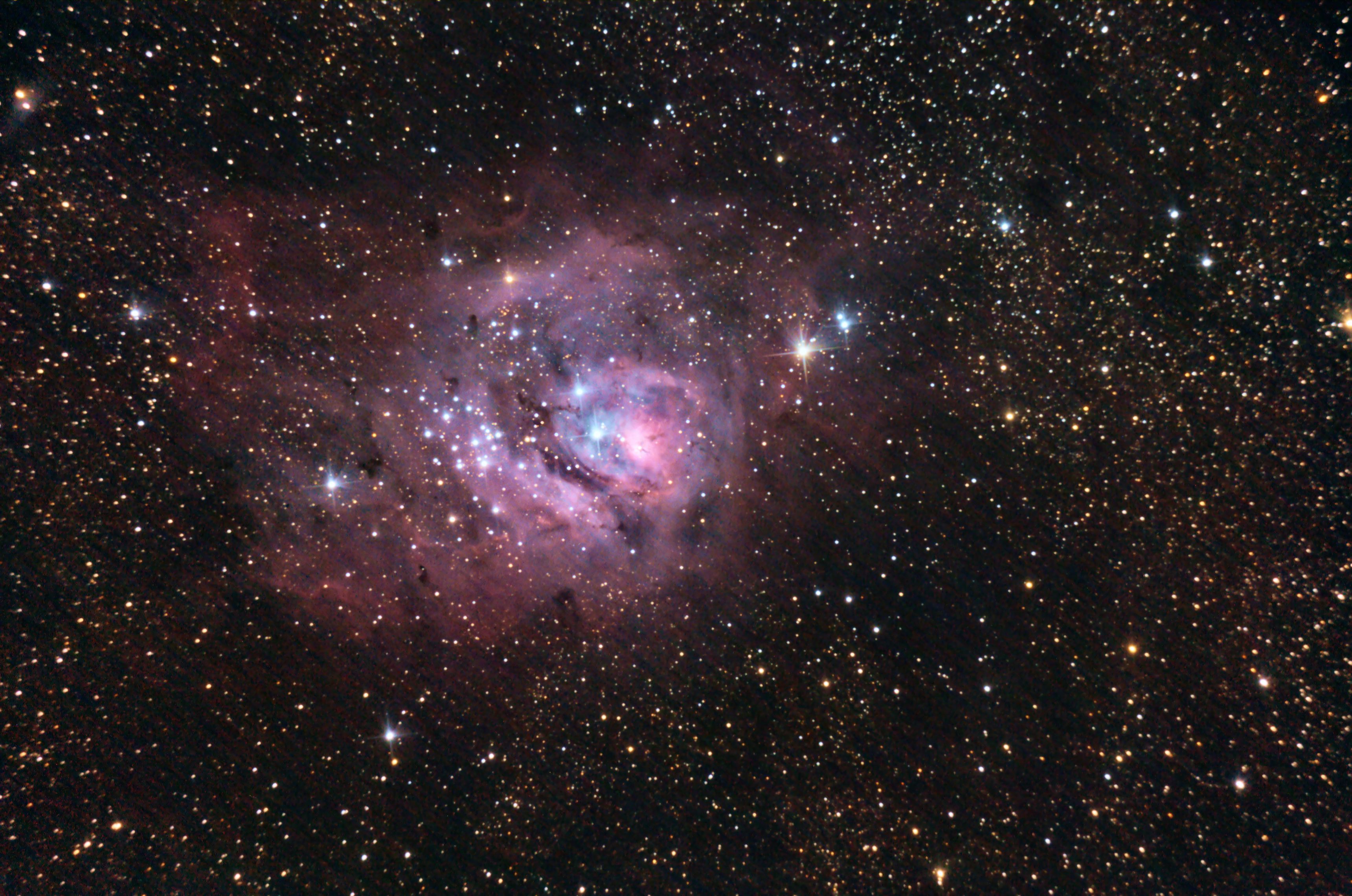
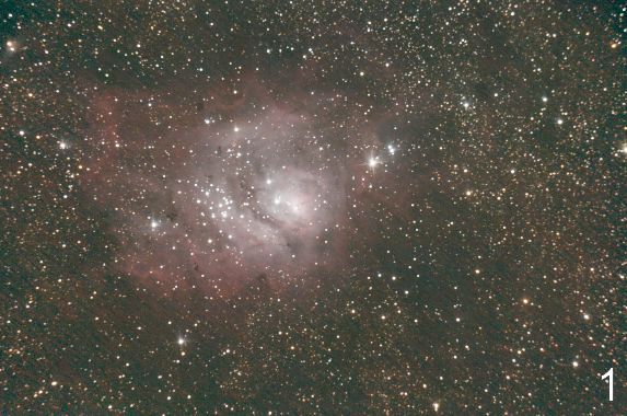
The contest was focused on a picture of M8 taken on a quite light polluted sky: this image is an example on how PixInsight could be great on dealing with such problematic pictures.

These the technical data of the image:

Image credits Martin Liersch (Google+ Profile)

M8, the Lagoon Nebula, on 2014/07/18. Equipment:

SkyWatcher EQ-6
Celestron C6N
Canon EOS 1000D
Tracking, no guiding

62 Light frames
60 sec exposure
ISO1600
40 Dark frames
21 Bias frames

 

The tutorial focuses on different issues:

• Dealing with sky gradients: ABE - DBE
• Color calibration 
• Denoise at linear stage: MMT
• Deconvolution for motion blur correction
• Correction for atmospheric chromatic aberration in DSLR or OSC
• From linear to non linear: HistogramTransformation - CurvesTransformation
• Boosting the color saturation
• Increasing Contrast: LocaHistogramEqualization

 

Beginning

Let's start opening the stacked image in the working space of PI: 

 

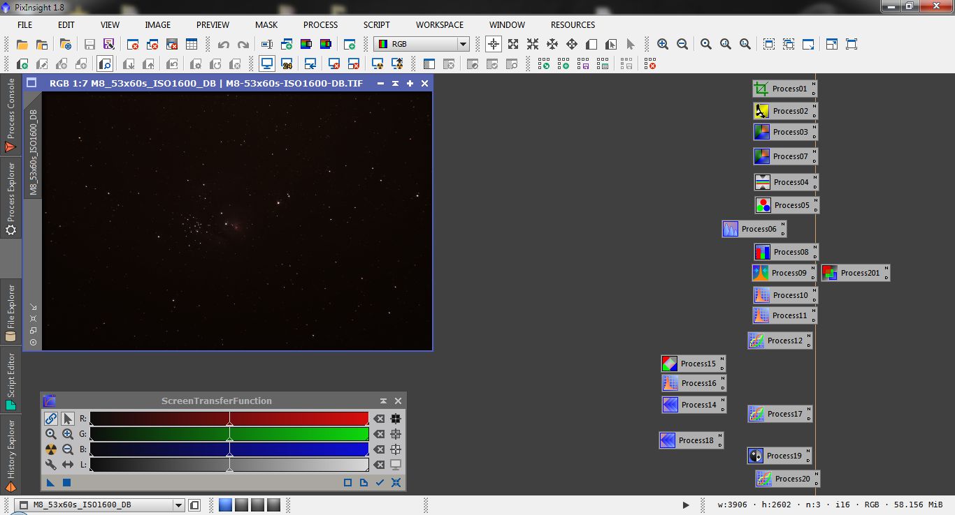
As usual, since the image is still linear, the nebula is barely visible so let's apply an automatic ScreenTranfert function clicking on the Nuclear button of the STF process:

The image is not modified by the process: the histogram transformation has been applied only to the screen representation of the image so the real data are still in linear form.

 

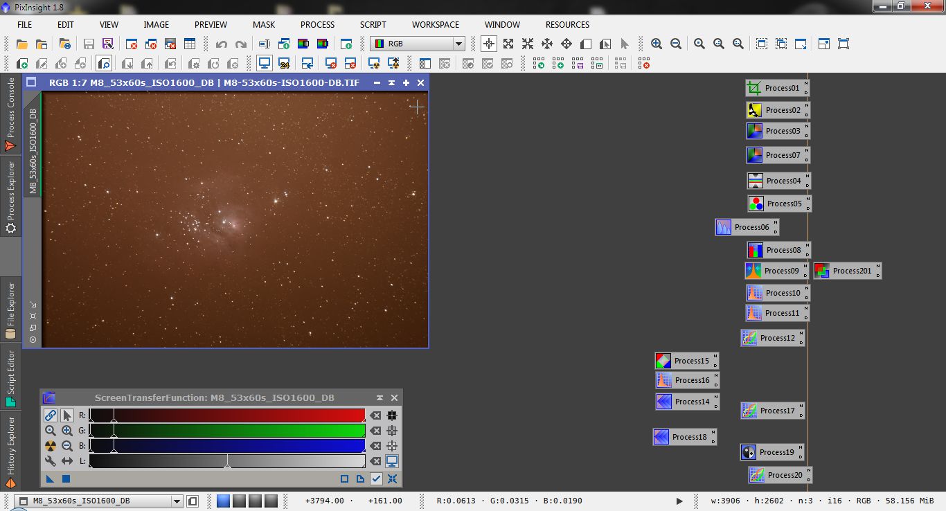
With the image so stretched we can easily see a few problems.

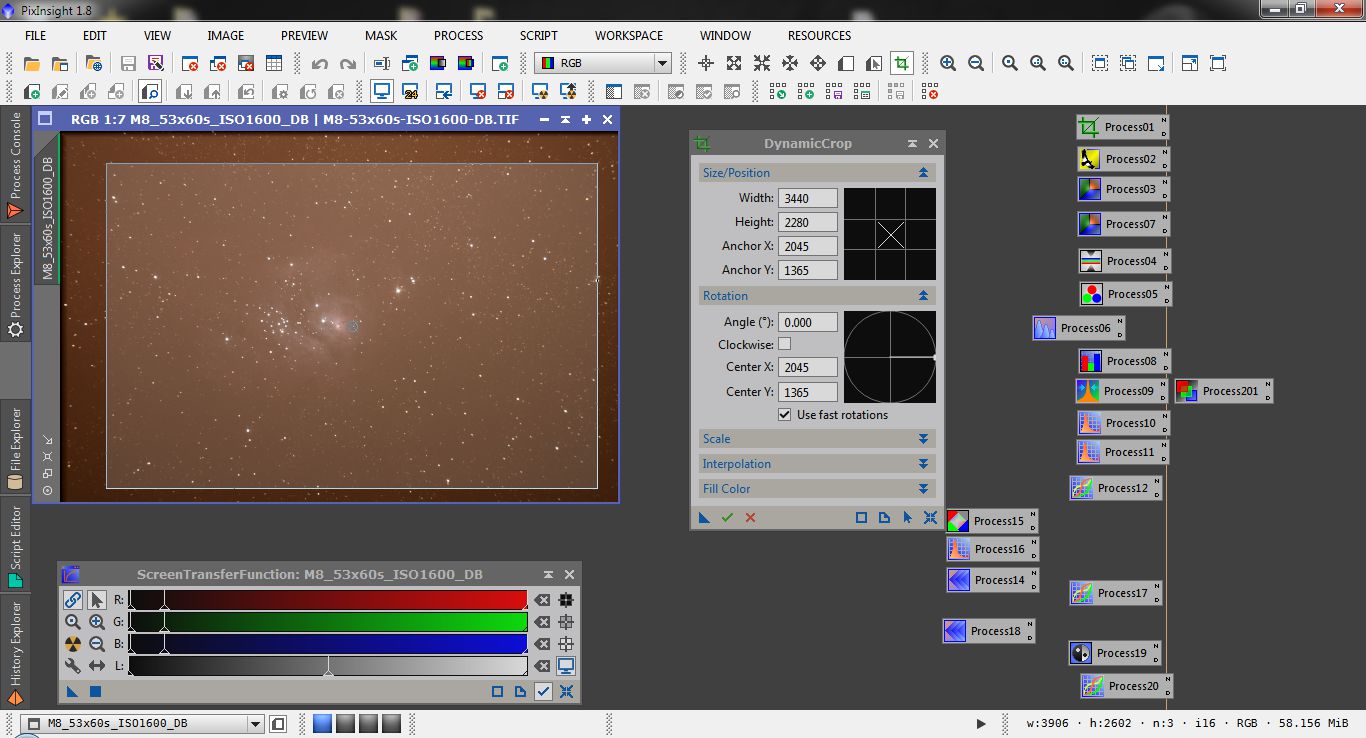
First we have to crop the image cutting away the borders where the single frames were not overlapping, then we will have to deal with gradients.

Let's start with cropping using the DynamcCrop process, selecting the desired area and confirm with the green V button on the process window.

 

Dealing with Background

Analizing the image it seems that the gradients come from two different sources:

1. An almost linear gradient from the bottom to the top of the image (light pollution?)
2. A nearly circular pattern almost centered in the frame (lacking of flat field?)

 If the interpretation of the gradient sources is correct than the first component is additive the second is mutiplicative.

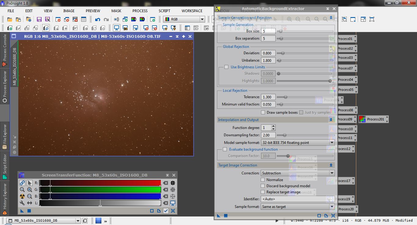
To correct the first source let's use AutomaticBackgrounExtractor with the default parameters except for tolerance in local rejection section (set to 1.3 instead 1.0) and Function Degree in Interpolation and Output section (1 instead 4).

the latter parameter is very important: setting the degree of the polynomial to 1 creates a smooth linear gradient.

Since the source of the gradient is additive let's use subtraction as correction method

  

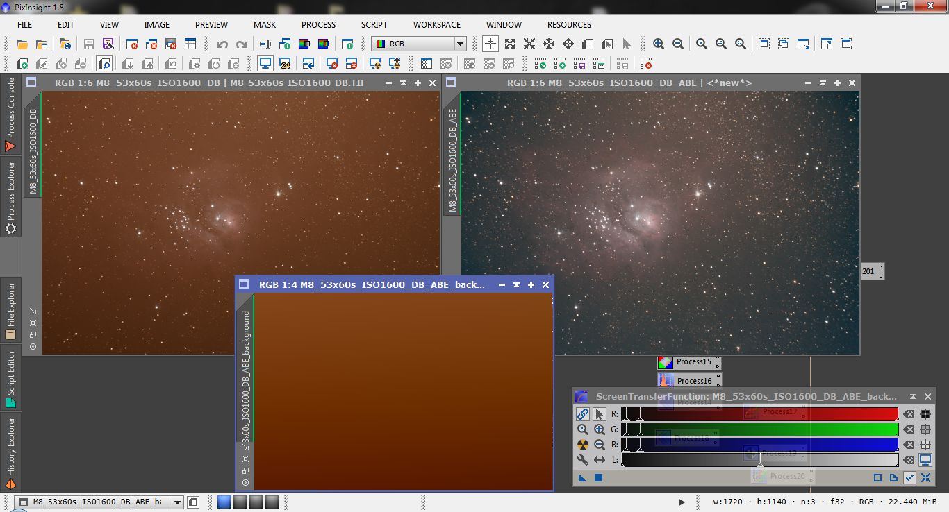
Here the generated background and the corrected image

  

Now we have to deal with uncorrected vignetting: for this task we will use DinamicBackgroundExtractor.

Let's put a few samples all around the center carefully avoiding nebula's faintest parts: since the background is so uneven, we need to increase tolerance in Model Parameters (1) section to 1.0 (instead the default od 0.5)

Since the vignetting is a multiplicative factor let's use Division as correction method.

  

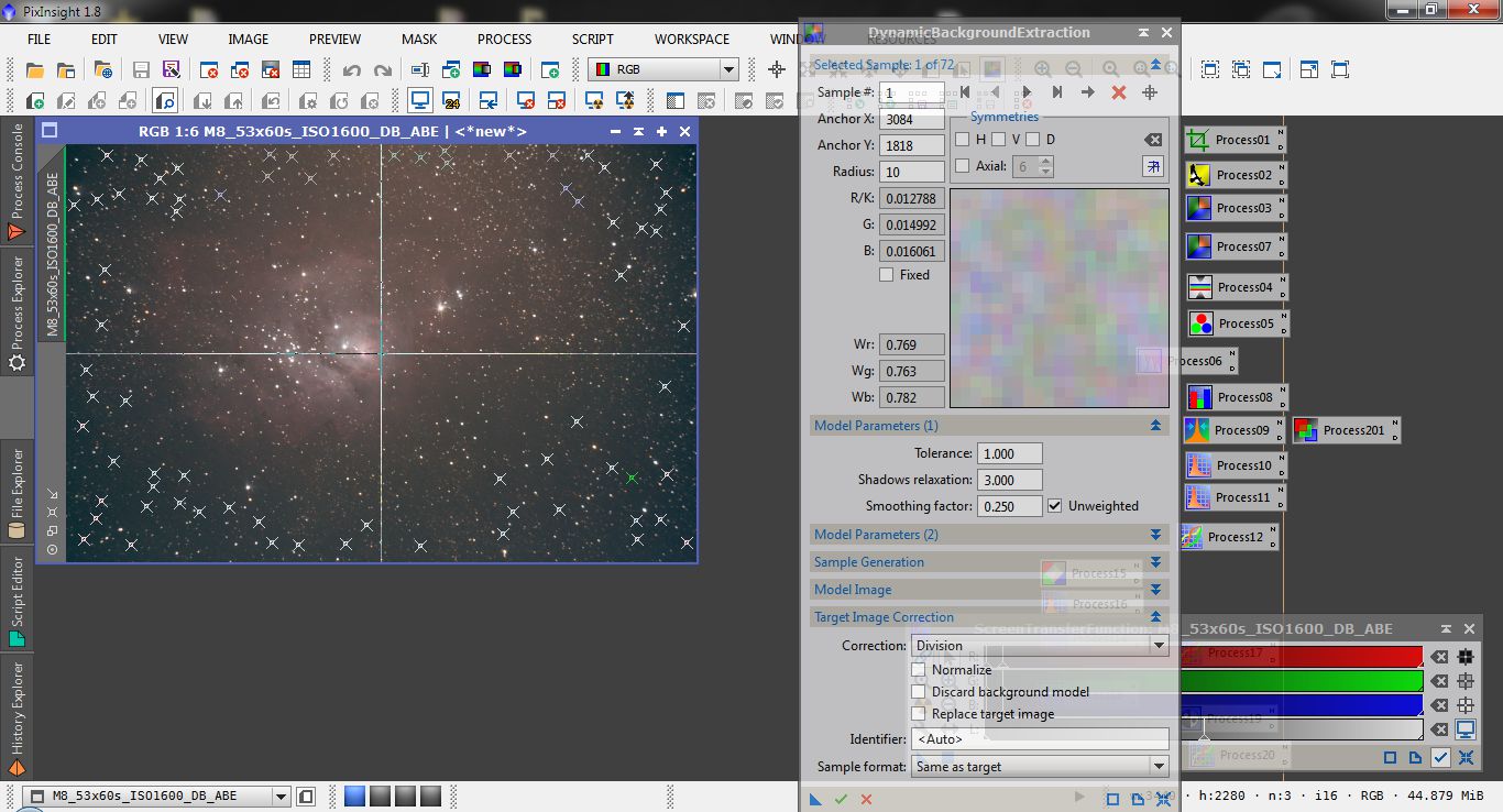
Here the generated background and the corrected image

  

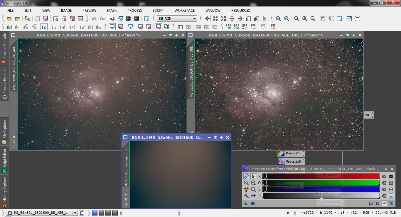
Now the sky is flat and we can contine with the next step.

Color calibration

In PixInsight color calibration is a procedure in two steps and, to work properly, should be performed at linear stage.

The first step is backgrond neutralization: since in this image we have done the background correction, background neutralization is not really necessary, but I prefer to do it though. 

Create a few previews around the nebula where the sky is dominant then use the script PreviewAggregator in the Utilities group that will aggregate the desired previews in a single image that can be used as a background reference then open the BackgroundNeutralization process.

 

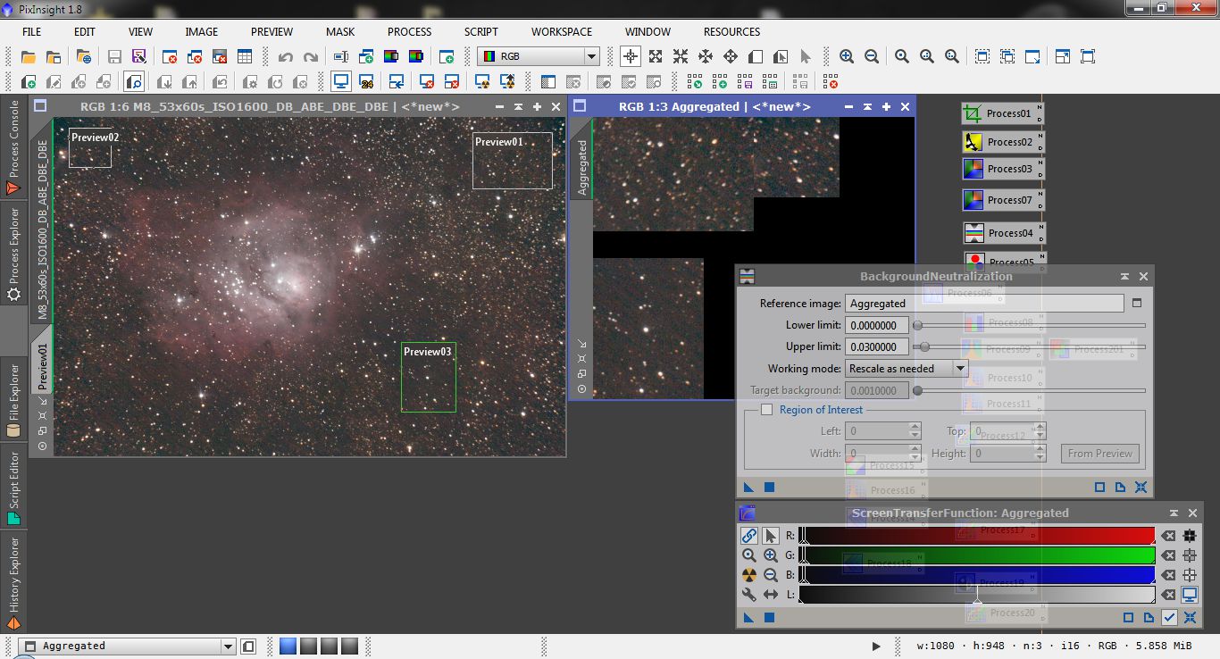
Note that the upper limit was set to 0.03 that is a little bit higher than the median value of the background.

Also note that the reference image is Aggregated.

Apply the process dragging the blue triangle over the nebula: now the background color should be neutral in color.

The Aggregated image no longer represent the background (that was neutralized in the original image) so we don't need it anymore: close it without saving.

 

Now it's time to color balance: to do that we need to use the process ColorCalibration with a white reference and, again, a background reference.

Since we have a lot of stars in the field we can use them as a white reference on the whole image.

As background reference we will use the same previews used for neutralization: let's use again the script PreviewAggregator to create the Aggregated image.

This image is different then the former one because the background was neutralized in the meanwhile.

Here the settings for the ColorCalibration

 

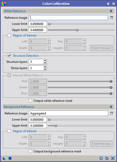
Note that the white reference image is blank (all the target image will be used), The upper limit is set to 0.44 to exclude from the white reference the saturated cores of the stars, Structure detection is active and the Reference image is set to Aggregated.

As usual apply the process to the image of the nebula.

 

Mouse over on the next image to see the Before calibration-After calibration comparision

 

 Denoise

 

Since this image was taken under a light polluted sky it is quite noisy especially in the backgound.

PixInsight has many tools for noise reduction both on linear and non linear stage; one of my favourite is MultiscaleMedianTransform (MMT).

MMT is a very flexible and powerful tool that can be used both in linear and non-linear stage; the latest release has also a built-in linear masking feature that helps the photographer to apply the denoising only where it is needed.

I will reduce the noise in the first three wavelet layers as in the following image

 

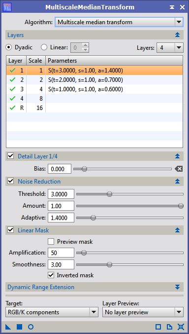
Note that the linear Mask option is activated with an amplification factor of 50 

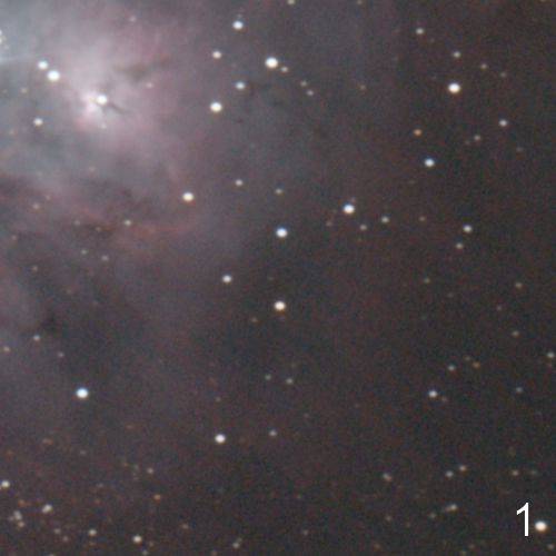
Mouseover on the next image to see a before-after denoise comparision

 

Deconvolution

 

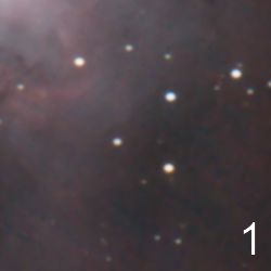
The image shows a slight motion blur due probably to a small inaccuracy in tracking: this problem can be corrected with Deconvolution.

Deconvolution has to be performed on linear data, this image is RGB therefore the deconvolution will be applied to the Y channel of the CIE XYZ color space.

Since the standard RGB working space was applied to the RGB image, the CIE Y channel is not linear so the first, very important, step is to change the working space parameter using the RGBWorkingSpace process.

 

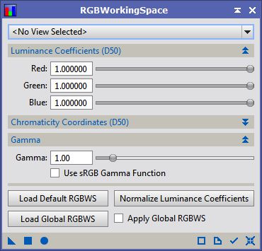
Here the three Luminance coefficient are all the same at 1 and, very important, the Gamma parameter is 1 so the CIE Y channel will be linear:

Let's apply the changes dragging the blue triangle icon over the RGB image.

Now we're ready to apply the deconvolution with a motion blur PSF

 

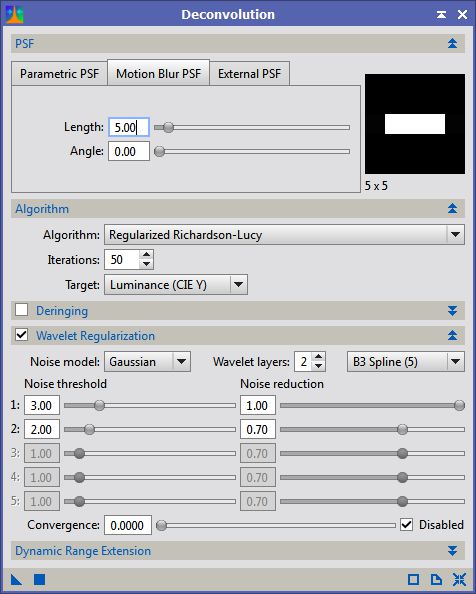
Te lenght of 5 and the 50 Iterations was found by trials and errors.

Mouseover on the next image to see a before-after deconvolution comparision of the star shapes

 

Atmospheric Chromatic aberration correction

 

Since atmospheric refraction index varies with wavelength, the air works like a prism, especially when an object is low: this effect creates in color cameras a blue halo above the star and a red halo below.

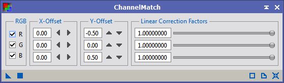
This effect can be corrected using the ChannelMatch Process that allows to move the three RGB channes independently.

Here we only need to move the red channel slightly up and the blue one slightly down: the correct shifts can be found by trials and errors

 

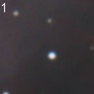
Mouseover on the next image to see a before-after Matching comparision of the star colors

 

Going nonlinear

 Despite all the work done, the image is still linear, so the nebula, in the original data, is almost invisible: it's now time to apply a nonlinear histogram transformation.

We will use a combination of HistogramTransformation and CurvesTransformation processes to enhance nebulosity without boosting too much the background

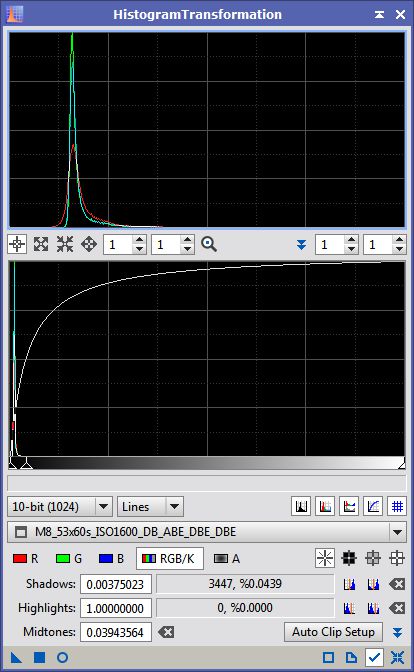
Opening the HistogramTransformation and CurvesTransformation make sure to activate the V checkmark in the lower-right part of the window in order to show the histogram of the active image.

First HistogramTransformation step

  

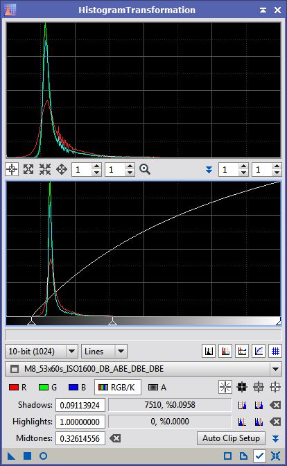
Second HistogramTransformation step

 

 

CurvesTransformation step

 

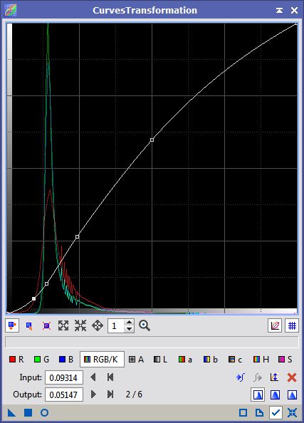
When doing Histogram transformation make sure to not to clip data on the right and left sides of the histogram or you will loose precious information.

 

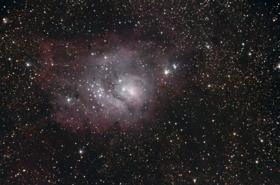
At the end of the process the image will look like the one below

 

Boosting the saturation

CurvesTransformation tool can be used for boosting the color saturation , anyway the saturation can't be boosted indiscriminately on the whole image because in the backgroun hides a very strong coloured noise.

We need to build a mask to protect the background boosting the saturation only on the best S/N areas: 

 

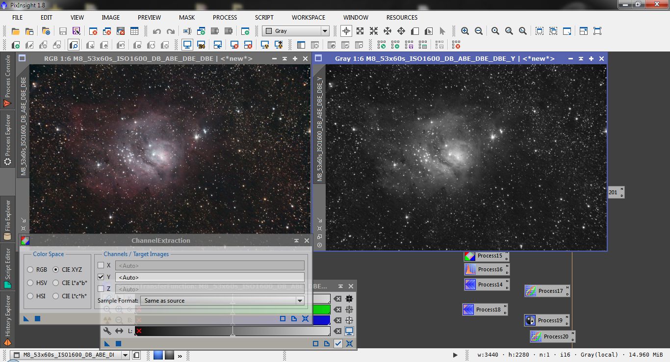
Extract the Luminance (CIE Y) channel using ChannelExtraction process

 

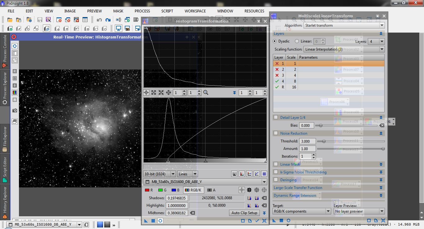
 Let's protect  more the background clipping the right end of the histogram and lert's smooth the mask removing the first three wavelet layers with MultiscaleLinearTransform

  

Finally the mask has to be applied to the image with the menu item MASK-Select Mask or simply by dragging the mask tab (on the upper left side of the image) over the image tab: when done the image tab color turns to brown to show that the mask has been applied  and the protected areas of the image turn red.

Since the mask visualization hides the image below, whe can hide it using the menu item MASK-Show Mask

to enhance the Saturation we will use CurvesTransformation on the masked image

  

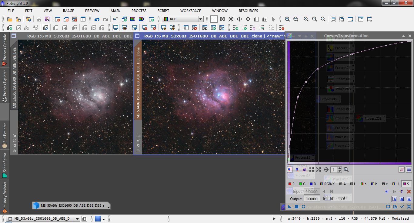
As can be seen on the above image, in CurvesTransformation, we selected the S (saturation) channel using a curve steeper on the left side boosting the saturation more in the low saturation areas and acting more gently in the areas where saturation is already high.

 

Increasing contrast

 

 As a final step we want to give a little bit more life to the nebula increasing contast between the lighter and darker areas.

PixInsight gives a lot of tool to achieve this goal, like HDRMultiscaleTransform or MultiscaleLinearTransform

Here we will use LocalHistogramEqualization.

This tool is very aggressive, mainly on the background where it tends to increase the noise a lot, therefore is better to protect the darker areas with a suitable mask.

Our goal at this stage is to apply the process only to the nebula without touching the stars and, mostly, the background.

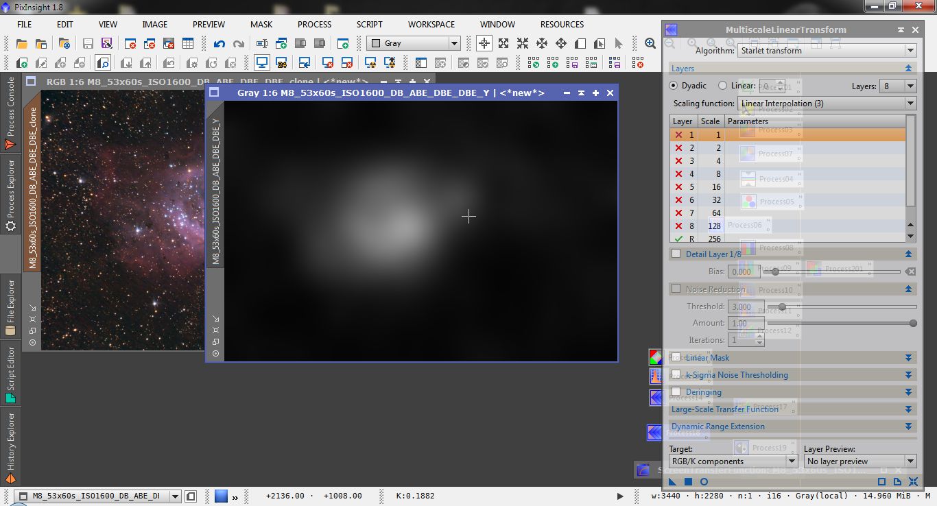
We can easily create such a mask modifing the Saturation mask created during the previous step and removing all the first eight wavelet layers: only very large structures will survive after the application of the process.

  

Since the mask was already applied to the image we don't need to do it anymore.

Now we can apply the LocalHistogramEqualization process

  

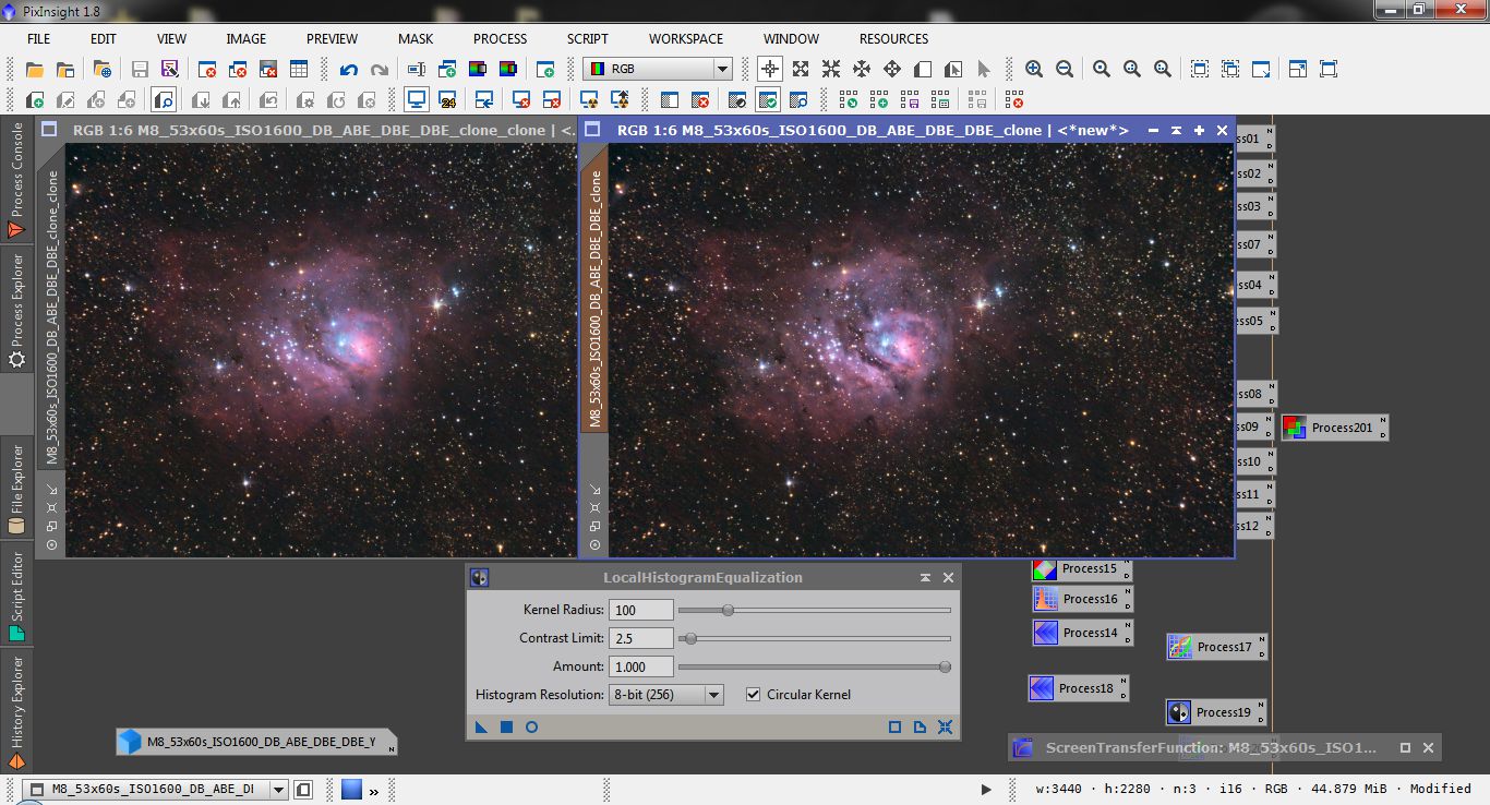
The Kernel Radius parameter controls the size class of the details that will be enhanced, the contrast limit defines how strong the process will perform: this parameters has to be found by trials and errors.

 

The final touch

As a final touch, after removing the mask, we can fine tune the curves again with CurvesTransformation process

and here the final result: Click for the full resolution version.