


Many of the astrophotographers of my generation, after passing through analog photography, approached digital astrophotography for the first time thanks to CMOS sensors.
Only a few, in fact, could afford the first cooled CCD sensors for astronomy: they werw expensive, small and difficult to use, reserved for professionals or advanced amateurs.
At the beginning of the 2000s, however, began to spread the first digital cameras at affordable prices for the general public and the astrophotographers began to use it to image the night sky.
These digital sensors, based on CMOS technology, certainly did not have the rigorously scientific imprint and dynamic range of CCDs, but they did allow to acquire quality digital images at a fraction of the price of a cooled CCD.
In thes way began my adventure in digital astrophotography: after a brief interlude with webcams (the legendary Vesta Pro and its little daughter Toucam), in 2008 I switched to a Canon 350D, modified with a Baader filter to extend the range in red.
However, my final goal, was to purchase a monochrome CCD equipped with color and narrowband filters, so shortly after I switched to SBIG CCD Camera.
In recent years, however, the trend is changing: CCD technology has reached a certain maturity and has no longer shown the great evolution of the first years, conversely CMOS technology has continuously evolved, filling the gap with CCD.
This why I was very curious to try one of the new CMOS sensors for astronomy.
The opportunity came thanks to Marco Rigo - Astrottica who gave me the current ZWO flagship: the color version of the ASI 6200.
On paper, the ASI 6200 is a small technological jewel:
- Sony IMX455 backlit sensor.
- 35mm "full frame" format.
- Peak quantum efficiency of just under 90%.
- 16-bit analog-to-digital converter.
- 3.76 micrometer pixels.
- Resolution 9576x6388 pixels (60 Megapixel).
- Readout noise 1 - 3 electrons (depending on the GAIN setting).
What, frankly, I find particularly interesting is the backlit sensor technology that fix what has always been the greatest limitation of CMOS: the on-board pixel circuit that significantly reduces the useful surface (and therefore the quantum efficiency) .
In the IMX455 the photons hit the "back of the sensor" so there is nothing casting a shadow on the pixel stealing photons.
Another interesting feature of CMOS in general and of this camera in detail is the very low readout noise which allows to shorten significantly the exposure time of the single frames.
In high GAIN mode the camera has a readout noise of about 1.5 electrons which rises to 3 electrons for the low GAIN setting (for comparison a normal CCD has 9-11 electrons).
This gives the camera an effective dynamic range of 14 bits (which decreases as the GAIN increases).
An important note: like all ZWO CMOS cameras, the GAIN parameter can be set by the user, this parameter is similar to the ISO setting of digital cameras: the higher it is, the more the sensor output signal is amplified.
However, the GAIN setting does not affect the sensitivity of the camera (which is defined by the quantum efficiency) it only affect the signal amplification.
Furthermore, the GAIN setting should not be confused with the A/D converter gain (expressed in electrons / ADU): while the GAIN setting increases the A/D gain decreases, the exact relationship between the two parameters can be seen in one of the graphs on the technical sheet on the ZWO website (https://astronomy-imaging-camera.com/product/asi6200mm-pro-mono) .
This is quite confusing for people coming fron CCD where the gain is set by the producer.
The discussion about the correct GAIN and OFFSET settings is beyond the scope of this review, but I would like to give a personal opinion: in deep sky astronomical photography (for which this camera is designed) the GAIN or OFFSET values should be optimized in order to have the best image dynamics; I find it absolutely useless and, sometimes, harmful that the setting of these parameters is left to the end user.
It would be nice that, as in the case of CCD cameras, they were preset to optimal "factory" values by the producer, maybe offering a couple of predefined settings (such as high and low readout noise) but without leaving complete freedom to the user.
The general appearance
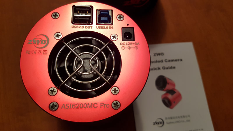
The camera has the classic appearance of ZWO sensors: a cylindrical aluminum chassis of a beautiful red color, very light but sturdy, on the sides there are the ventilation grilles, on the back there are all the electrical connections: the socket for USB 3.0 type B connection cable, two USB 2.0 sockets for connecting accessories (filter wheel, autoguide camera) and input for 12V DC power supply.
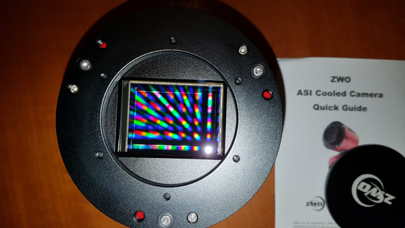
On the front, protected by an aluminum threaded cap, there is the large image sensor.
The standard equipment is completed by a flat type B USB connection cable, a pair of cables for connecting accessories and some threaded connecting rings.
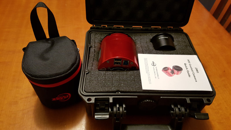
The camera was sent to me in a plastic case filled with precut foam rubber to protect it from bumps.
The thing that really surprised me was the absence of a power supply: only afterwards I discovered that the 12 V power supply is sold as an accessory.
Although the cost of such a power supply is negligible, I was very surprised by its lack, even if it is true that the camera can also be used without direct power supply, if you don't need cooling.
Having several power supplies at home, luckily I had no problem finding a compatible one, but it is something that must be taken into account when buying.
Another thing I didn't particularly like is the included connection cable: the length of this cable is about 1.5 meters: completely insufficient to reach my control PC when the camera is connected to the telescope.
Also in this case the problem is easily solved by purchasing a longer cable. (maybe the supplied cable is meant to be used on mini PCs mounted on the telescope, like the ASIair).
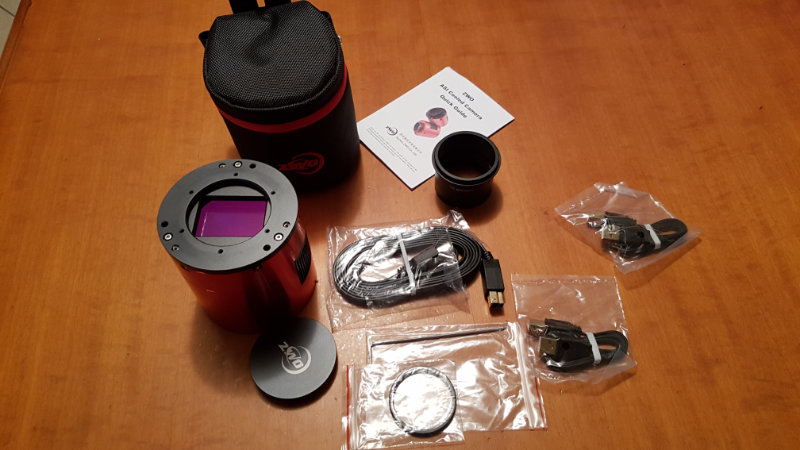
In addition to the power supply, in the basic equipment, a CD / USB stick with the camera control software was also missing: you must have an internet connection to download the latest versions of control software and drivers.
Bench tests
The installation of the camenra went smoothly and within a few minutes I was ready to do the first tests: given the cloudy weather I decided to proceed first with some "bench" tests.
As mentioned above, the camera must be powered at 12 V in order to activate the cooling through a Peltier cell which can cool the sensor down to -35 °C with respect to the ambient temperature.
As a first test, I therefore wanted to evaluate the cooling time of the chamber.
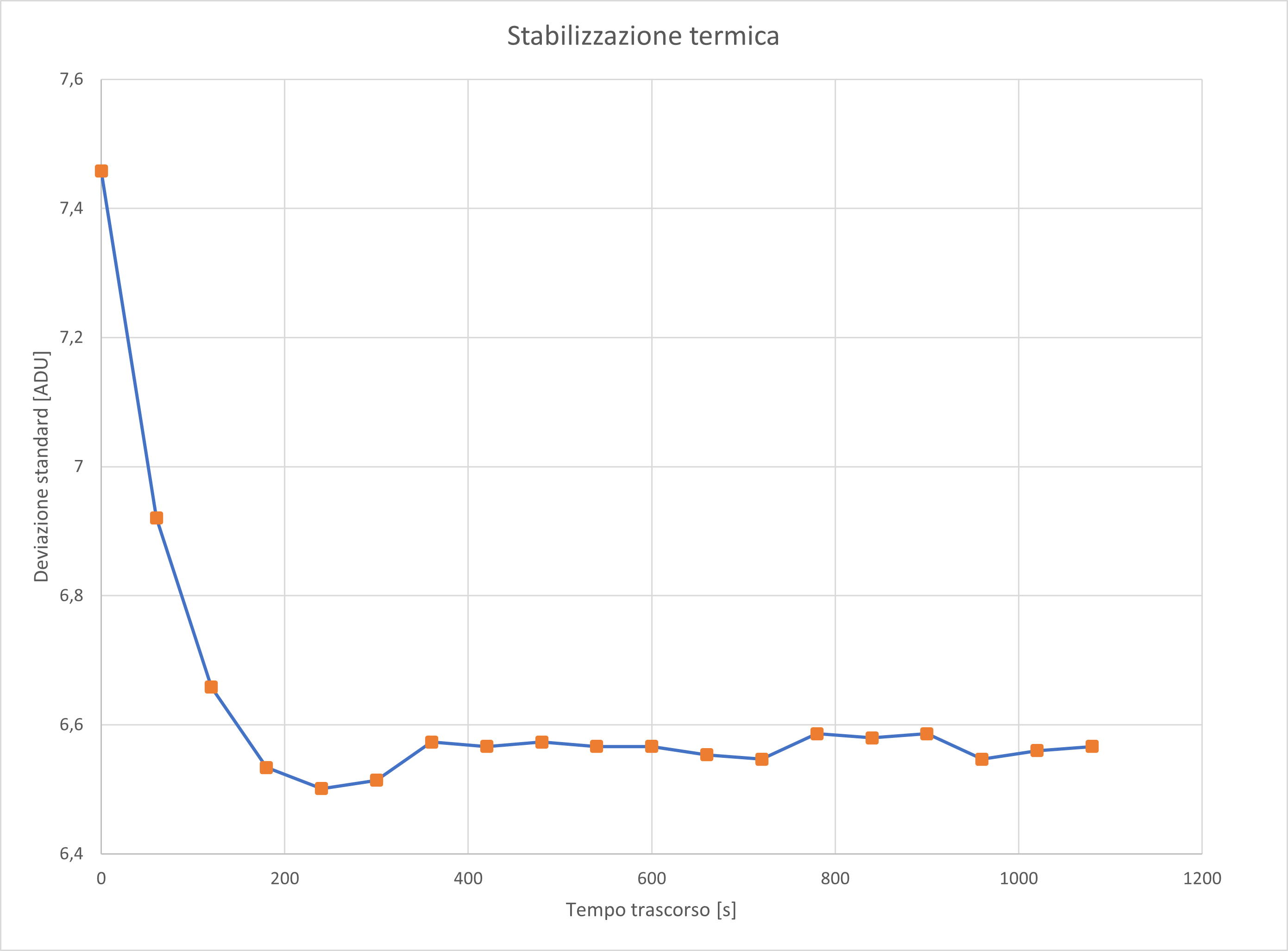
Not knowing if the camera was equipped with zero point compensation, I verified the achievement of the target temperature by evaluating the standard deviation in a 1000x1000 pixel frame in the center of the sensor, acquiring 30-second dark frames.
The idea underlying this test is that the colder is the sensor, the lower the dark current and therefore its standard deviation.
The sensor started at a temperature of 20 ° C and was cooled down to -5 ° C (therefore with a difference of 25° C compared to the theoretical maximum of 35°C)
As you can see from the graph below, the sensor cools down very quickly, falls below the set temperature, then stabilizes at the target temperature: the complete stabilization of the chamber takes place in about 500 seconds, after which the chamber can be considered stable.
On the cooling front I found one of the very few (probably the only noteworthy) flaws:
If the chamber is disconnected from the control software, the peltier cell immediately stops functioning and the sensor begins to heat up; given the low thermal inertia of the system, the heating occurs very quickly, causing a few minutes hiatus in the shooting session, to allow the system to re-stabilize.
In one case, after the camera was disconnected and reconnected, cause to my software management error, an oscillation in the temperature of about 2° C around the equilibrium point was triggered. to re-establish the right temperature it was enough to disconnect the chamber, let it heat up by about ten degrees and then cool it again. However, the phenomenon occurred only once.
The second test I wanted to do was on the quality of the dark frame.
Many CMOS cameras are subject to AMP glow: an electroluminescence phenomenon that produces areas with different illumination on dark frames; although the AMP glow can be completely corrected by good calibration practice, in some cases it can become annoying and leave visible traces on the final image.
Many of the ZWO cameras suffer from this characteristic, but the ASI 6200 is advertised as totally exempt from the phenomenon.
I then verified this statement by running some test darks at a temperature of -5 °C.
The behavior of the camera in these conditions was excellent: there is no trace of amp glow in the dark frames, the image is perfectly homogeneous, perfectly "flat", except for a certain number of hot pixels (perfectly normal) .
Furthermore, the dark current turned out to be extremely low, perfectly in line with ZWO declaration on its website (about 0.0019 electrons/s per pixel at -5 ° C).
After this first phase of introductory tests I decided to assess the linearity in the camera response.
CMOS cameras have the reputation of suffering large deviations from linearity, but often this information is not accompanied by objective data and is based on hearsay.
I was therefore particularly interested in testing the response of this sensor.
For the linearity analysis, in addition to the classic residual test on linear regression, I also used the local gradient test that I described in my previous article
(La verifica della linearità dei sensori d'immagine: andare oltre la regressione lineare. only in Italian): I recommend reading it before proceeding with the data analysis (eventually with the help of Google translate).
Unlike the Moravian camera analyzed in the article mentioned above, the ASI 6200 has a "rolling shutter": a completely electronic shutter, without moving mechanical parts, so problem of the shadow of the shutter on the sensor is completely absent and you also have more freedom in the choice of shutter speeds.
For the tests I collected three sets of data:
The data captions in the pictures are in Italian, but are quite easy to understand.
"Bassi ADU" series: acquired with times between 0.20 and 300 seconds with the light panel set to low brightness. Camera set to GAIN 0 and OFFSET to default value.
"Alti ADU" series: acquired with times between 0.20 and 300 seconds with the light panel set to high brightness. Camera set to GAIN 0 and OFFSET to default value.
"GAIN 100" series: acquired with times between 0.20 and 300 seconds with the light panel set to low brightness. Camera set to GAIN 100 and OFFSET to default value.
The shots were taken without any optic, simply using a cap with a hole of about 0.5 mm to illuminate the sensor.
For each shutter speed I acquired 5 shots, in order to calculate the average value and standard deviation of the measurement: the experimental uncertainty thus measured was represented with 1 sigma error bars.
Below are the graphs obtained from the analysis of the three data series.
As will be seen later, the analysis and interpretation of the data thus obtained is far from simple.
The first graph represents a direct comparison of the relationship between shutter speed and ADU
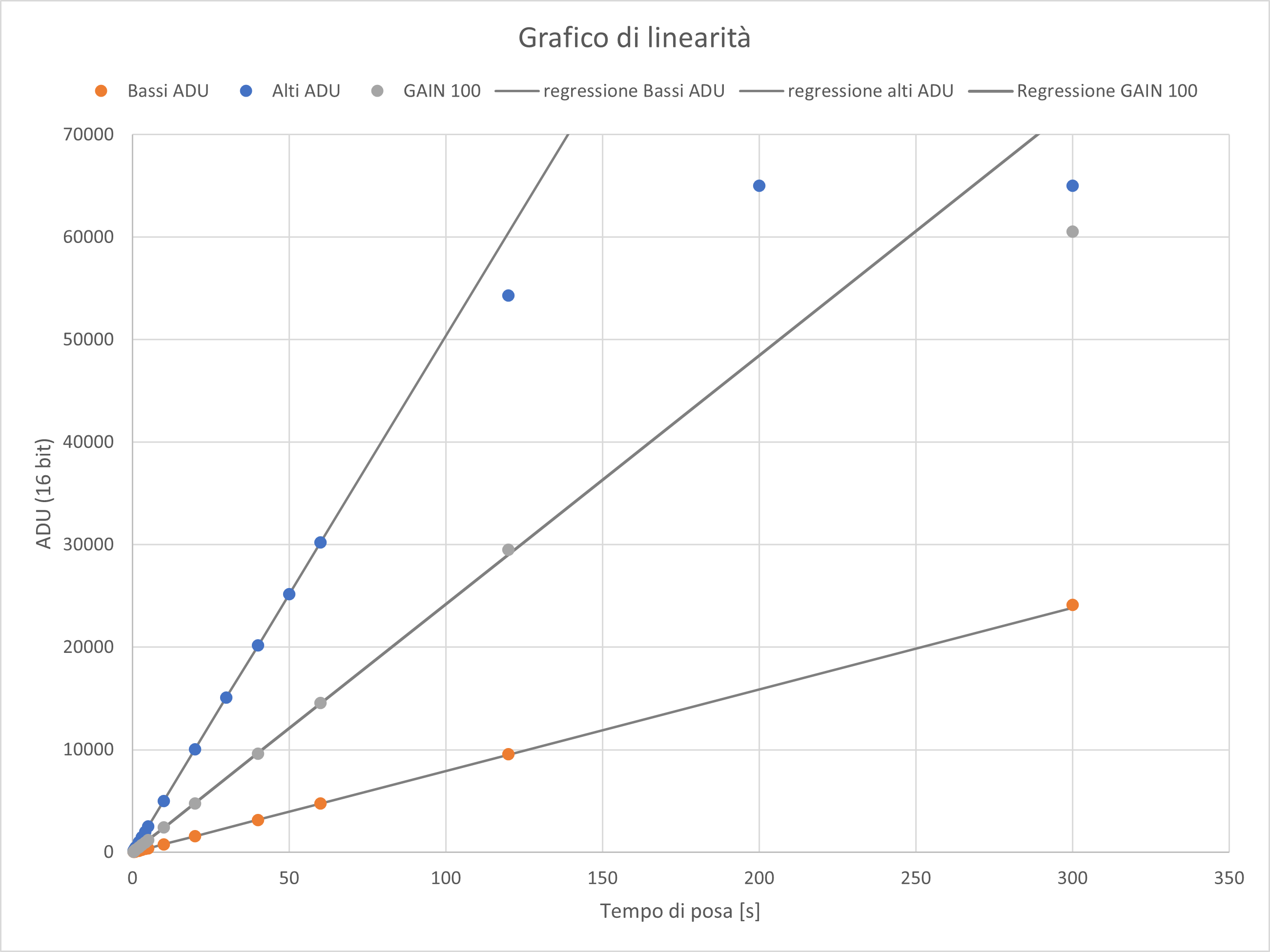
As can be seen, the behavior of the sensor is substantially linear until saturation occurs (very evident in the "Alti ADU" set).
The camera therefore behaves substantially as expected from a digital sensor, but this test is very insensitive to small deviations from linearity: this is why the analysis of the residual is necessary.
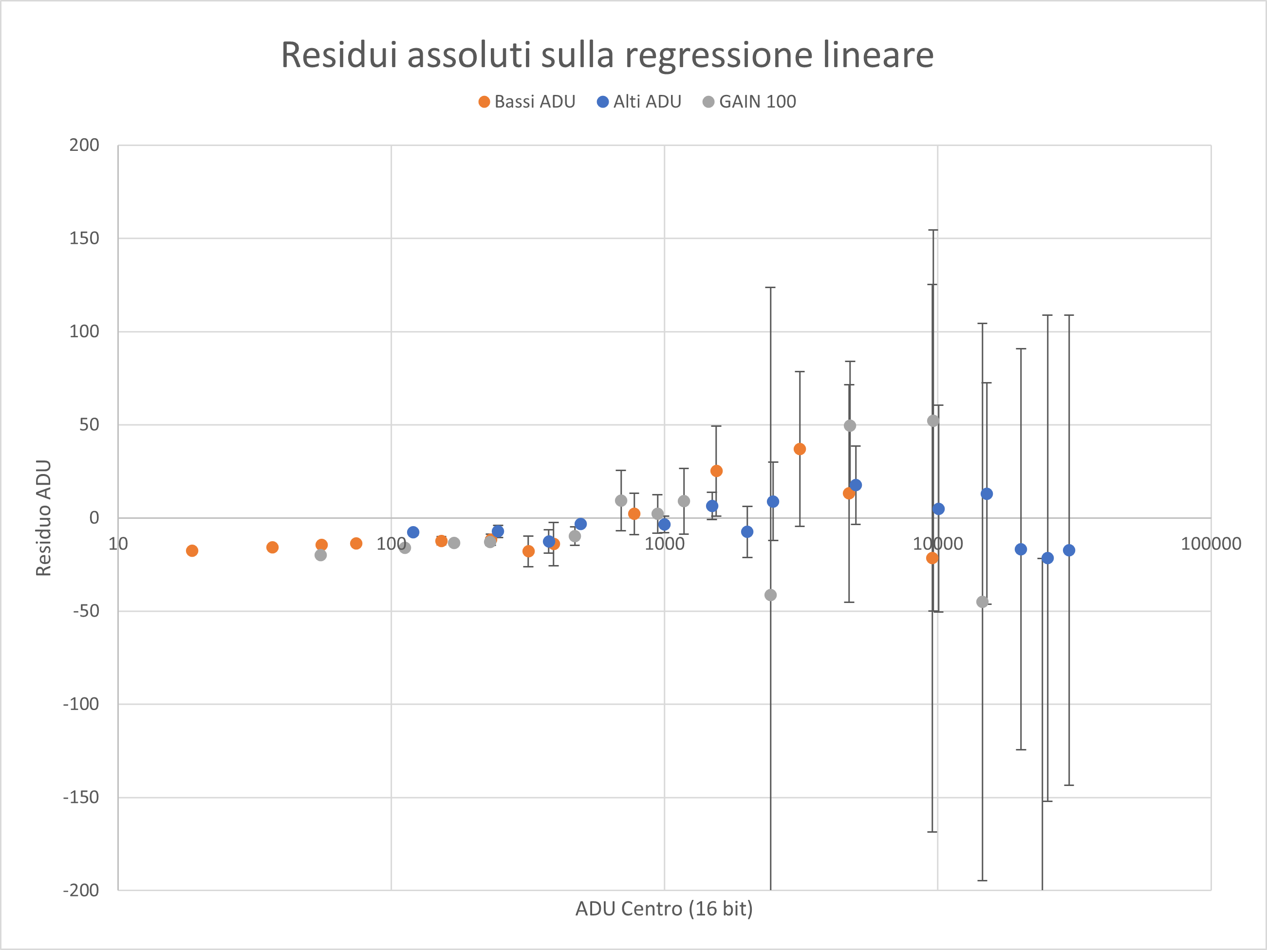
The linear regression calculation was carried out, for all data sets, using only the exposures between about 150 and 20,000 ADU, in order to exclude the saturation areas and the too short shutter speeds.
The following two graphs show the trend of the residuals both in absolute form (Theoretical ADU - Real ADU) and in relative form (percentage residues (Theoretical ADU - Real ADU) / Real ADU).
To better separate the data at low ADU (taken with very short shutter speeds) the abscissa axis has been represented in logarithmic form.
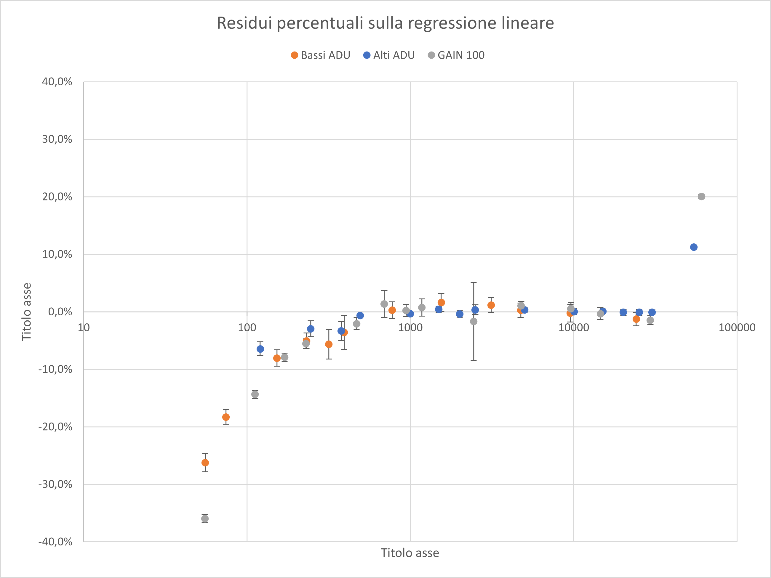
The most interesting graphs seems to be the second one (percentage residuals)
The first thing that can be noted is a significant deviation from linearity at low ADU (below 800), we will talk about this deviation later, but remember that the graph is in logarithmic form, so the apparently non linear region is very small.
On the other hand, the very interesting thing is that the sensor is perfectly linear (within the experimental error) in the range that goes from 800 to about 40,000 ADU, here the camera begins to deviate from linearity due to saturation.
It is difficult to determine where the deviation takes place actually.
To better characterize the visible deviation at low ADU I opted for the local gradient test, measuring the image in the center and near an angle and then calculating the ratio as described in the article cited above.
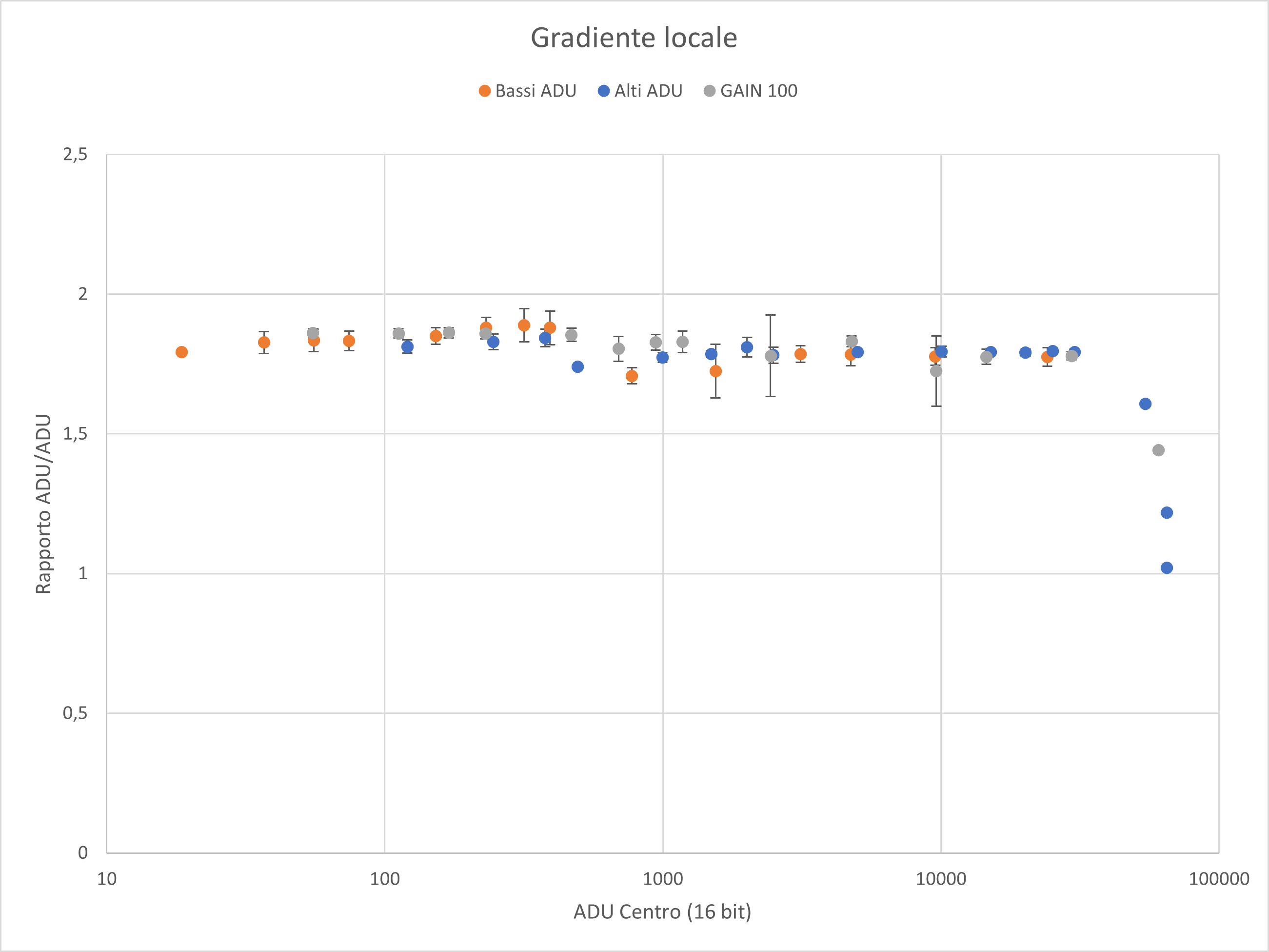
Comparing the graph of the percentage residuals with that of the local gradient we note that:
- It is confirmed that the deviation of the sensor from linearity occurs around 40,000 ADU (saturation).
- It is confirmed that beyond 1000 ADU the sensor is linear (the residuals are close to zero and the local gradient is flat).
- Around 800-1000 ADU there is a slight but significant disturbance.
- Before 800 ADU the sensor would appear linear again flat local gradient).
Giving an interpretation to these data is rather complicated: the data suggest that the sensor follows a certain linearity line at low ADUs (less than 1000) and that, around 1000 ADU, there is a sot of "knee" after which the sensor follows a second line with a slightly lower slope than the first.
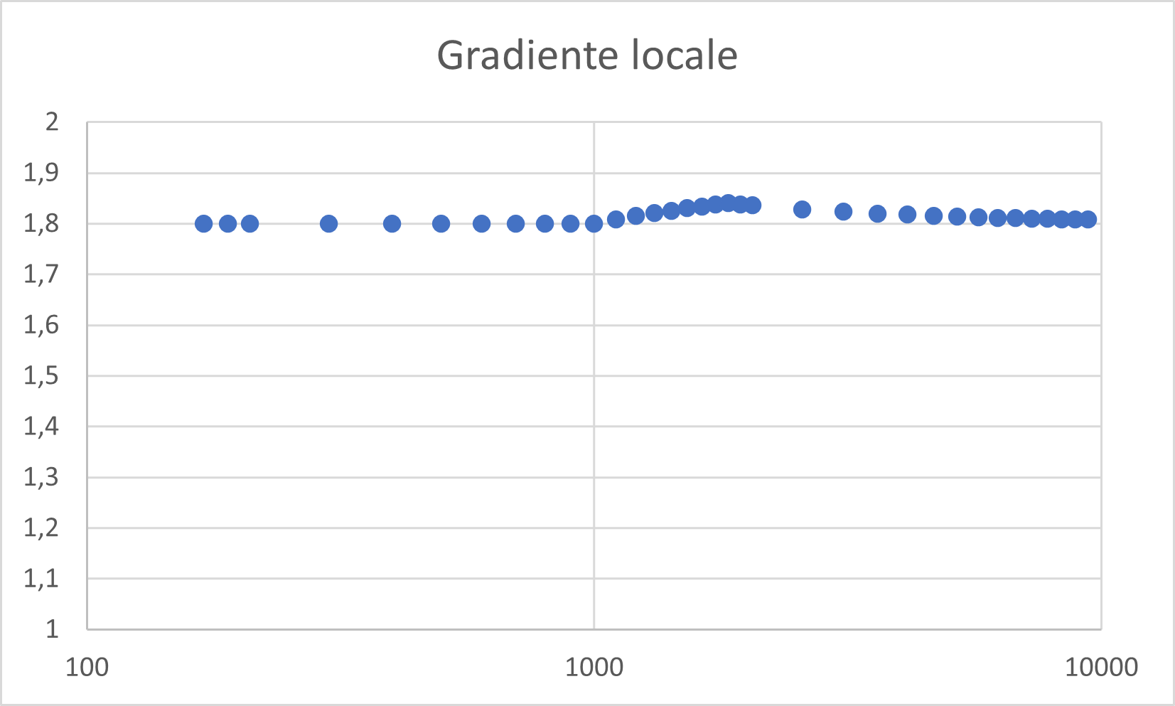
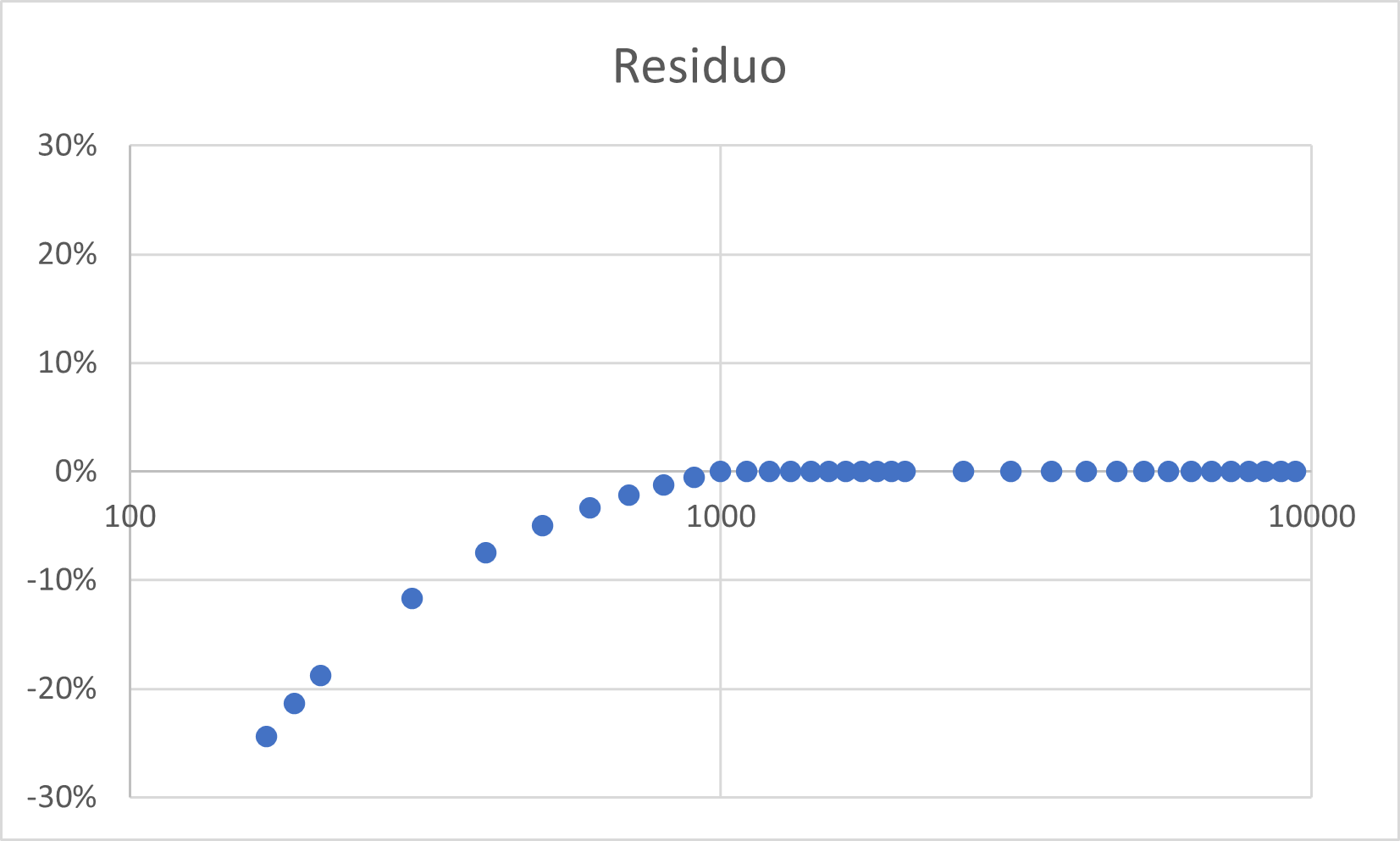
This interpretation seems to be supported by a numerical simulation obtained by varying the slope of the linearity relationship at 1000 ADU by 5%.
| Local Gradient simulation | Simulation of percentage residual of linear regression |
 |
 |
NOTA Importante:
This interpretation of the data is based solely on the mathematical examination of the graphs, unfortunately my knowledge of electronic sensors in general and CMOS in particular is not sufficiently thorough to know whether this explanation can describe a physically possible case or not.
Surely this behavior deserves an in-depth study, in order to understand if what is observed is a genuine phenomenon or an artifact due to a measurement error.
Although I consider this second hypothesis unlikely (since the phenomenon occurs in a similar way on three independent data sets), I cannot exclude that a systematic error in the measurement method may exists.
But the key question is: if such behavior were verified, would it prevent the camera from functioning properly?
The answer depends a lot on the intended use: The ASI 6200 has been designed for long exposure deep sky astrophotography.
In this context, theoretically, a non-linear behavior could make image calibration difficult.
In practice, however, given the minimal entity of the perturbation, I dont't think that this hypotetic deviation from linearity may have a negative impact in the use of the sensor in the astrophotography field.
This assumption was fully confirmed by field tests carried out under a city sky: the images was easy to calibrate.
Field tests
For real tests I connected the camera to my William Optics 110 FLT equipped with a Type IV flattener.
Unfortunately this reducer is not designed for full frame, therefore I was forced to crop the images due to the defects on the shape of the stars.
Obviously these defects are not to be attributed to the camera which has the only "fault" of being gigantic.
Its use proved to be very simple: as an acquisition software I use SGPro which controls the camera via Ascom driver.
The connection and management of the camera was immediate and stable: I used the the ASI 6200 for several nights without ever having connection problems.
Despite the 60 megapixels, the download of images is relatively fast thanks to the USB3 connection.
Here, however, one of the problems that accompanies this gigantic room has arisen: the size of the files.
A single 16-bit black and white shot reaches nearly 120MB!
The same file after debayerization (remember that the model tested is in color) occupies 360MB
The color master light saved in 32-bit XISF (PixInsight) format exceeds 720 MB and, if you use WeightenedBatchPreprocessing in Pixinsight (which saves in a single file the Master light and rejection maps), the final file reaches the stratospheric quota of 2 GB !!!
It is therefore clear that anyone wishing to buy this "toy" must have a PC with great computing capacity and, above all, fast and reliable storage.
Furthermore, not all the pre-processiong and post-processing software are capable of handling such a large amount of data.
Personally I use PixInsight 1.8 for all file processing operations: with this software I had no problems in processing , but the cooling fans of the CPU of my PC made me understand the workload to which the poor guy was subjected.
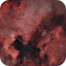
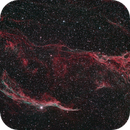
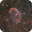
The tests were initially carried out in integral light, then, given the light pollution that characterizes my area, I preferred to apply an Optolong L-eNhance filter (also kindly lent by Astrottica).
The results can be seen on my Astrobin gallery.
| Un mosaico a due pannelli della regione di NGC 7000 | Il Velo del Cigno | La nebulosa Crescent in luce integrale |
 |
 |
 |
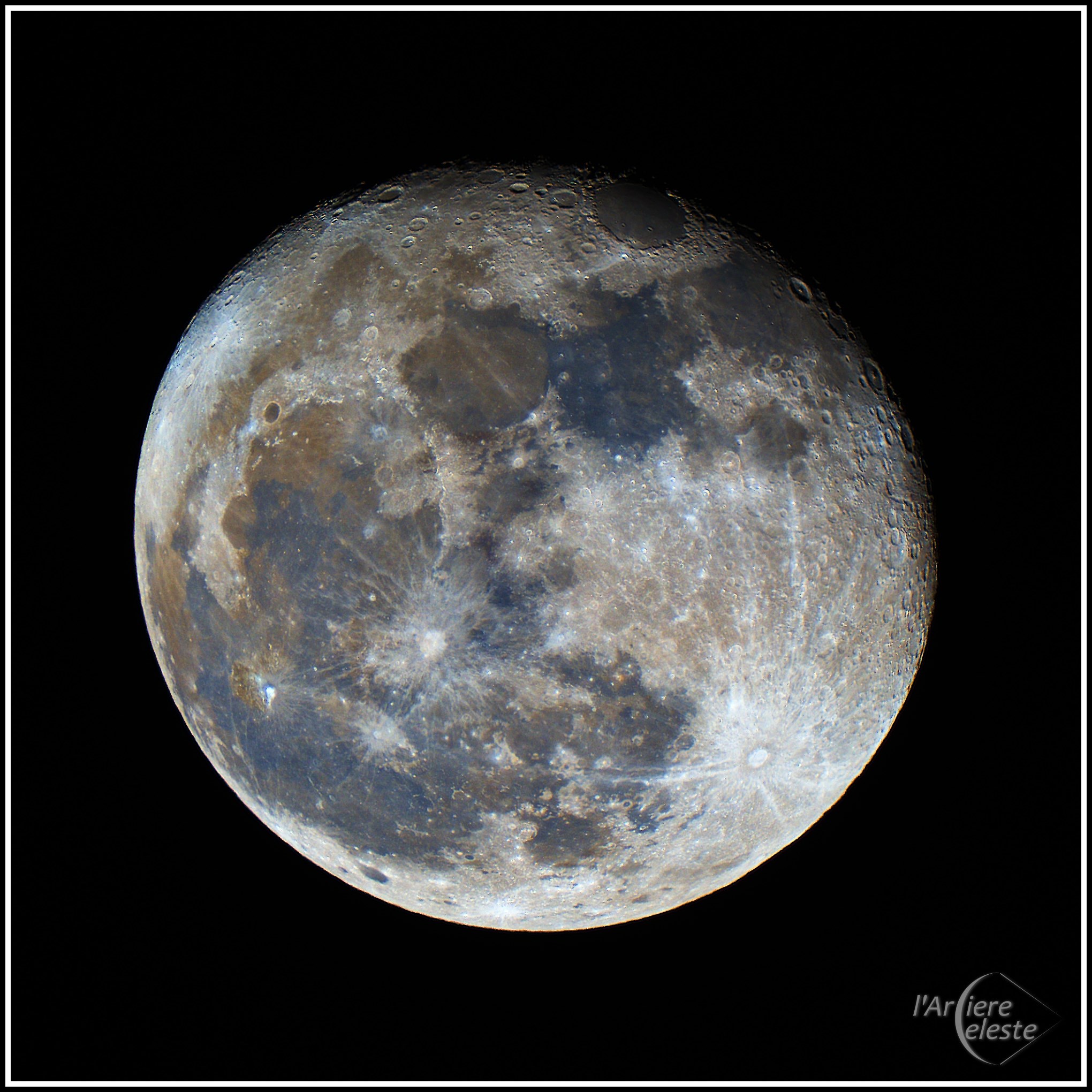
As a last test I wanted to test the capabilities on the planetary imaging.
The electronic rolling shutter allows you to shoot with very short shutter speeds, suitable for bright subjects such as the Moon.
The image was obtained with the same configuration as the deep sky images and a single shot with a shutter speed of only 30 thousandths of a second.
Conclusions
The ZWO ASI 6200 turned out to be an extraordinary camera characterized by a very low readout noise, an almost non-existent dark current and a very high quantum efficiency.
The linearity test highlighted a possible anomaly around 1000 ADU which however does not seem to affect the correct functionality of the camera.
On the field it has proved to be a reliable and versatile tool.
The only drawback is the impossibility of maintaining the set temperature once the chamber is disconnected from the control software.